N1 - Stellar spectra of different spectral types (BACHES)

The aim of this observation is to obtain an overview of different spectral types. Thus, we will give you the coordinates and the apparent magnitude of four stars of different spectral types that are well visible during the night of your observation. Take spectra of these stars in order to classify them by means of the spectral lines and the shape of the continua. From the deviation of the absorption lines in the spectra from their rest wavelength, you can calculate the radial velocity of the star towards or away from us by using the Doppler effect.

Nightly observations at the OST in Golm with the BACHES echelle spectrograph are required. The scientific and technical background for this observation is presented in the seminary talks. A list with objects will be provided by us.

Note: The following exposures are needed for every star:

• the stellar spectra
• darkframes for the stellar spectra
• at least one calibration spectra with the build in ThAr calibration lamp

and only once:

• at least three calibration spectra with the continuous flatfield lamp
• darkframes for the continuous light source

The QHY268M camera should be operated with 2×2 binning!

The calibration exposures are needed to calculate the pixel scale (wavelength calibration) and to remove the instrument signatures and possible artifacts.

The first tasks are to login to the Laboratory Computer and to copy the observational data (FITS files), including darkframes, and the additional calibration exposures from the directory ~/data/<date> to your own directory ~/data_reduction/. It is recommended to perform the data reduction of each star in an individual directory. Furthermore, it will be necessary to sort the acquired images into subfolders according to their category: darks, flatdarks, flats (images of the continuous calibration lamp), thorium argon (ThAr), and star images. A possible folder structure could look like this:

 Star_1/
    Darks/
    Flatdarks/
    Flats/
    ThAr/
    Star_1/
 Star_2/
    Darks/
    Flatdarks/
    ...

Note: This folder structure is essential for some data reduction steps. It is therefore essential that the files are sorted accordingly!

There are different tools to view the FITS files (two dimensional CCD images or data tables). ds9 is easy to handle and can be started from the terminal via:

 ds9 filename.fit

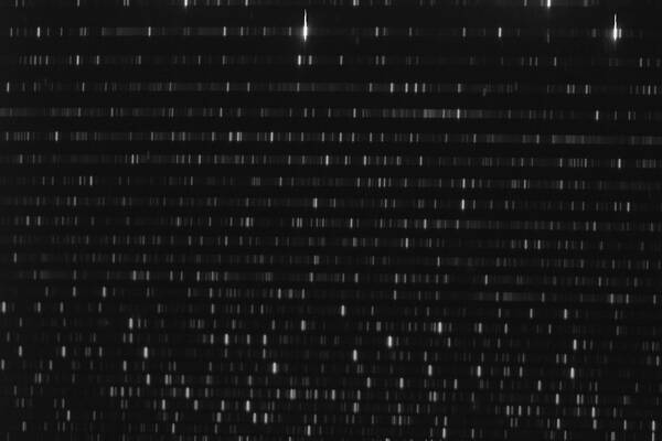
The next step is to check the orientation of the exposures. The correct orientation is crucial for the final result, since the data analysis software expects that the wavelength is increasing from the lower left to the upper right of the image (2D spectrum). The best image to check the orientation is the exposure of the thorium argon lamp (ThAr lamp), which can be compared with the example below. If the image is flipped, you will need to correct the orientation of all images that are necessary for the data reduction.

ThAr exposure (ST-8) as it should appear in ds9 and MIDAS

Some modules from the OST photometry pipeline are required for the data reduction. Python modules should always be installed in a virtual environment to reduce dependency issues. A virtual environment can be created using

 mkvirtualenv ost_photometry

By doing so, we have named the virtual environment ost_photometry. The fact that we are in the virtual environment is indicated by the string '(ost_photometry)', which now precedes each terminal line. To leave the virtual environment, simply type

 deactivate

If you want to reconnect, you can do so by typing

 workon ost_photometry 

This is also necessary if you reconnect to a12, e.g. after a break, and want to continue the data analysis.

The OST photometry pipeline can then be installed in the terminal using pip as follows

 pip install ost_photometry

All necessary dependencies are also installed in this way.

The scripts for the data reduction can be found on the lab course computer in the folder ~/scripts/n1_baches. Copy the script 1_masterimages.py into the local directory where you want to analyze the star (e.g. Star_1). This script will create among other files the masterdark and the masterflat needed in the following processing steps. Furthermore, this script stacks all star images, if more than one was taken during the observations. It also offers the possibility to bin the observed images, if this was not done during the observation. It also cuts not needed parts of the captured images. This simplifies the further analysis steps. Last but not least, you should specify in this script if the exposures have to be mirrored (see previous step), so that this can be corrected as well. The configuration area of the script looks like this:

 ############################################################################
 ####           Configuration: modify the file in this section           ####
 ############################################################################
 
 ###
 #   Path to the directories with the images
 #
 #   Darks:
 path_darks = '?'
 
 #   Flat darks:
 path_flat_darks = '?'
 
 #   Flats:
 path_flats = '?'
 
 #   Thorium Argon exposures:
 path_thorium_argon = '?'
 
 #   Spectra:
 path_spectra = '?'
 
 #   Output directory for the reduced flats. The master files will be saved in
 #   the current directory.
 out_path = 'output'
 
 ###
 #   Flip images? Possibilities: True and False
 #
 flip_images = False
 
 ###
 #   Bin the images? Possibilities: True and False
 #
 bin_images = False
 
 #   Binning factor
 binning_value = 2
 
 ###
 #   Trim images to remove non essential parts and thus simplify MIDAS handling
 #   Possibilities: True and False; Default: True
 #
 trim_image = True

In path_darks, path_flat_darks, path_flats, path_thorium_argon and path_spectra the corresponding subfolders are to be entered, which were created in section Preparations. out_path is the directory where the script places intermediate results. The reduced files (master_dark.fit, master_flat.fit, master_thar.fit, master_spectrum.fit) are stored in the local directory so that they are more easily available for the following analysis steps.

If you want to mirror the recordings you have to set flip_images to True. If the images should also be binned, set bin_images to True. The binning factor can be determined via the variable binning_value.

Important: When the data reduction is finished, disable the virtual environment with

 deactivate

The data reduction will be performed with the MIDAS software package that is developed by the ESO. A lot of information on MIDAS can be found in this manual.

Note: MIDAS may be installed from the standard package repositories if you want to perform the data reduction on you own computer. But two of the routines have to be adjusted, otherwise MIDAS runs into an error. The routines can be provided by the supervisors.

MIDAS can be started from the console with

 inmidas

The scripts necessary for the data reduction of BACHES spectra are loaded via

 set/cont baches

By means of a leading $ sign also the default commands of the bash shell (like ls, cd, …) can be executed within the MIDAS shell.

The identification of the individual orders, the identification of the emission lines in the ThAr spectrum, and the correlation between the pixel and the wavelength scale is performed by the MIDAS script calibrate/baches. The call could look like:

 calibrate/baches master_flat.fit master_thar.fit 26 26 24

The five parameters have the following meaning:

1. Flat field: name of the flatfield exposure – give here the master flat field exposure
2. Calibration lamp: name of the ThAr exposure – give here the master ThAr exposure
3. Num. of orders: number of orders to identify (recommended default: 26)
4. Slit order width: width of the orders in pixel (recommended default: 26)
5. Slit extraction width: width of the area within the orders in pixel that should be extracted (recommended default: 24)

The first two parameters are obligatory. The parameters will be printed on the screen after the execution of the script:

 PARAMETERS FOR THIS CALIBRATION:
 ===============================
 Flat field  = master_flat.fit
 Calibration lamp = master_thar.fit
 Calibration table = thar.fit
 Num. of orders  = 0026
 Slit order width = 0026
 Slit extraction width = 0024
 Offset from center slit = 0.00000E+00
 Tolerance on RMS = 1.00000E+00
 Polynomial degree  = 0004

By means of this list, the parameters can be checked once more. In most cases, the default values can be used for the additional parameters that are not listed in the command above.

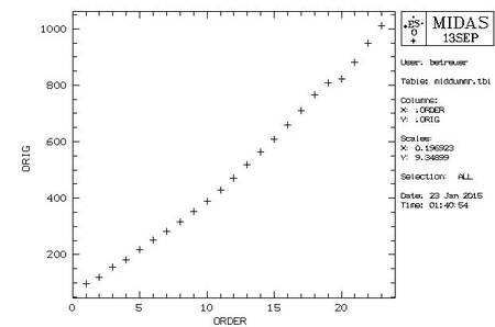
The program starts searching for the individual orders on the flatfield after a confirmation with y. The largest number of orders that can be recorded with the ST-8 is 24, which is also the default of the search algorithm. However, the flux in the blue is often not high enough that the automatic identification can successfully find the orders with the two shortest wavelength ranges. If the script is not able to find the number of orders that are specified in Num. of orders, the following text will be printed to the terminal:

|**************************************************
 ****  Warning: Defaults in the order detection ***
 ****   Table middummr.tbl has been plotted     ***
 **************************************************
 *       Read the help of DEFINE/HOUGH,           *
 *       Section: In Case of Emergency            *
 **************************************************
 * If you modify interactively middummr.tbl,      *
 * restart later with DEFINE/HOUGH P4=FOLLOW      *
 **************************************************
 * Now you can:                                   *
 *  1 - Go on                                     *
 *  2 - Stop here                                 *
 **************************************************

Furthermore, the following chart will be displayed in an additional window:

In this case, the script should be stopped by entering a 2. Afterwards the script can be restarted with a reduced number of orders, e.g.:

 calibrate/baches master_flat.fit master_thar.fit 23 20 20

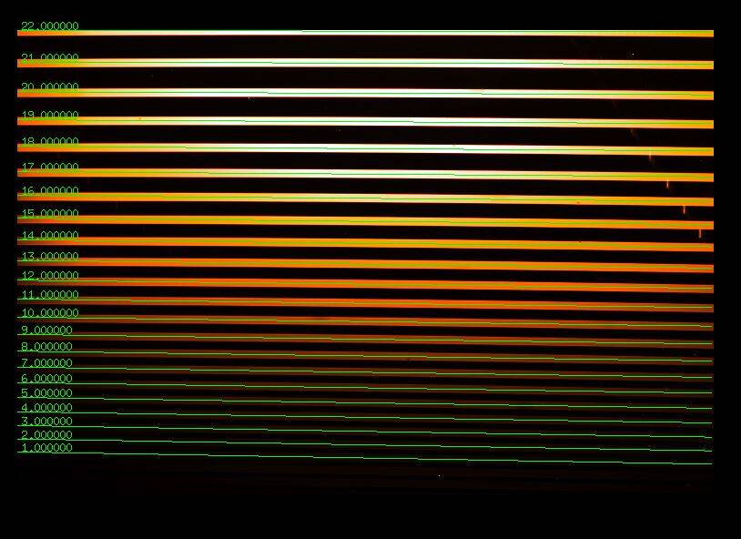
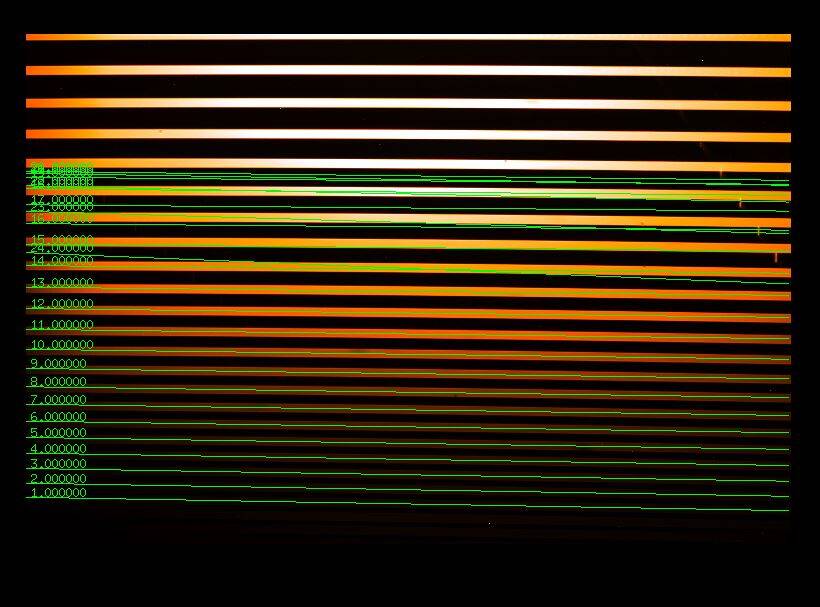
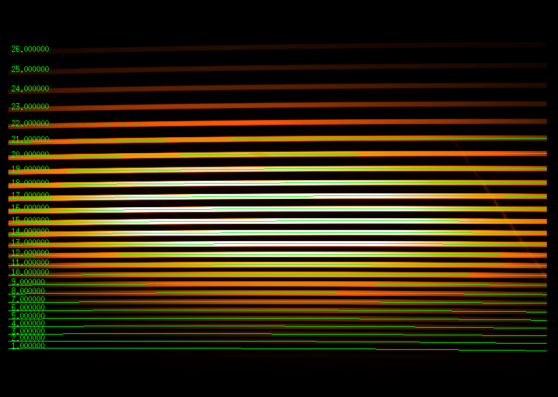
A solid method is to gradually reduce the number of orders until the script executed successfully. Afterwards, the flatfield with the identified orders will be displayed in an external window (see below). It should be checked whether the marks of the orders are horizontal and whether they coincide with the actual orders that are visible on the flatfield. The left figure shows a successful test run, whereas the middle figure depicts a failure. The right figure shows a flatfield image taken with the QHY268M, where it can happen that MIDAS does not finish drawing all identified orders. From the order numbers, however, it can be assessed if all orders were successfully identified or not. The numbers also depend on whether the images are binned. As we usually use 2×2 binning, the above values should suffice. In case we have used 1×1 binning for the spectra however, you might have to double the second and third value.

Successful identification of the orders

False identification of the orders

Identification with the QHY268M

Apart from the number of orders, the width of the orders (Slit order width), and the width of the area within the orders that should be extracted (Slit extraction width) needs to be specified. The default values of 20 pixel are only with restrictions applicable to our combination of BACHES and ST-8. Therefore, these parameters need to be adjusted on a case by case basis.

Troubleshooting: You may get the error output

(ERR) Problems in executing /usr/lib/eso-midas/1SSEP/stdred/exec/necdef.exe

The cause of this error has not yet been clearly identified. This error could be caused by the brightest order being at the edge of the image. Try cropping or adding additional pixels to the image. Note that you will also have to crop or expand all other images accordingly.

After the identification of the orders is completed, the wavelength calibration can be started by entering y.

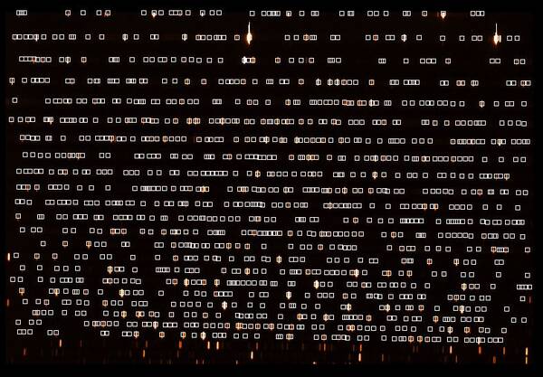
In the first step of the wavelength calibration, the script is searching for those emission lines of the ThAr spectrum that lie within the identified orders. With our instrument setup, the script should be able to find more than 1500 lines for the 50μm or 25μm slit, respectively. If this number is not reached, the sharpness of the ThAr exposure is probably insufficient. Once the identification of the lines is completed, a window that looks similar to the following figure should be displayed on the screen. Each white box is a line recognized by MIDAS.

ThAr spectrum, where all identified lines are marked

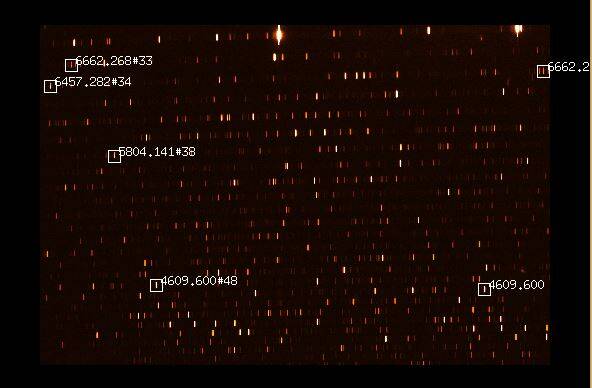
After another confirmation with y, two line pairs need to be marked on the ThAr spectrum, so that the script is able to correctly identify the emission lines and to determine the overlap areas of the orders. One line pair should be in the red and the other one in the blue wavelength range. The following two lines prove to be useful: 6677.282Å and 4609.6 Å. Alternatively to the first line the 6457.282 Å or the 6662.268 Å can be used. This might be necessary if MIDAS has not recognized a line. In this case, the corresponding line in the figure above is also not marked by a white box. To facilitate the localization of the lines, an additional window will be displayed (see below), showing some example lines.

ThAr spectrum with some example lines

Compared to the example shown above, there are usually significantly more lines on our images, because our camera chips are larger than the ones used to create the figure above. For example, the 6677.282Å is not highlighted at all here. This line is the bright line to the right of the 6662.268Å. This becomes clear on the following figure, on which the two pairs of standard lines are labeled.

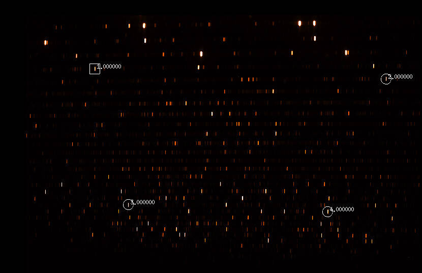
On a corresponding graphic in MIDAS these line pairs have to be marked by mouse in the given order. If necessary the size of the selection box for the lines can be adjusted with the arrow keys on the keyboard. It is important that the lines are marked in a continuous sequence. After the four lines are marked, the selection needs to be confirmed with a right click into the window.

ThAr spectrum with the two marked line pairs

Afterwards, the order number of the first marked line, the wavelength of the first line pair, and the wavelength of the second line pair need to be entered. If the default line pairs have been marked (as shown above), the first line will be in the 33rd order. The wavelength of this line is 6677.282Å. If the 6457.282Å is used, the order number is 34. The second line pair is at a wavelength of 4609.6Å. At the end, the terminal should look like this:

 Enter absolute order number of first pointed line (square mark) : 33
 Sequence no. 0001, Order no. 0033. Enter wavelength : 6677.282
 Sequence no. 0003, Order no. 0048. Enter wavelength : 4609.6

It is sufficient to give the order number of one line, since the others can be easily calculated by the software. In the next step, the script is automatically searching for a wavelength solution.

Troubleshooting

   *** Sorry. Cannot identify feature 0002 ***

 
 *** Initial, coarse estimate ***
 Mean pixel width      : 9.99039E-02 wavel. units
 RMS error of relation : 1.37550E-01 wavel. units
 Maximum allowed error : 9.99039E-02 wavel. units
 This accuracy appears insufficient to attempt automatic line identification.
 Please check your identifications.
  *************************************************************
  *             Wavelength Calibration Diagnosis              *
  *************************************************************
  *          Linear fit of : m * lambda = b * xr + a          *
  * A = 218935.70420 B=      3.89221 RMS =       29.363       *
  *************************************************************
  *    Parameter    *    Value    *    Optimum   *    RMS     *
  *************************************************************
  *    Order number *       33    *        33    *      29.36 *
  *  Rotation angle *    -1.95540 *     -2.97270 *      10.35 *
  *  Binning factor *     1.00000 *      1.23330 *      10.35 *
  *  Ident. 1 and 2 *  6677.28200 *   6682.09003 *       9.36 *
  *  Ident. 3 and 4 *  4609.60000 *   4606.28318 *       9.36 *
  *************************************************************
 However the accuracy may be still acceptable.
 Start anyway (y/n, default no) ? 

Afterwards the flatfield correction may be prepared. To do this, answer the following query with y:

 Do you want flat correction [yn] (y)?

In addition, a calibration of the flux can be performed using a standard star. This option is usually not used in the lab course. Therefore, the corresponding query:

 baches_calib: Do you want to correct flux with a standard star [yn] (y)?

can be answered with a n.

The next query regarding the blackbody correction can in turn be answered with y:

 baches_calib: Do you want to correct flux with master_flat as a blackbody [yn] (y)?

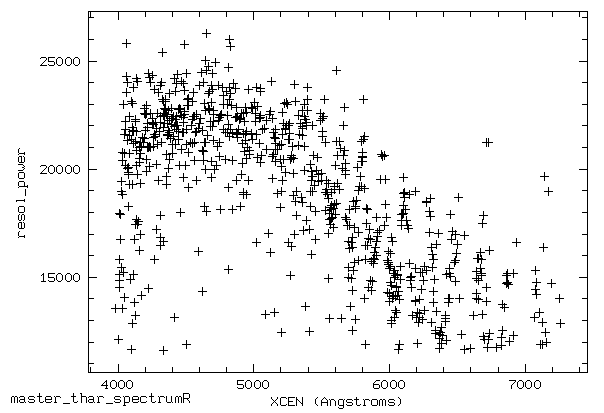
In the last step of the calibration process, the average resolution can be calculated and a figure illustrating the resolving power ($R = \frac{\Delta \lambda}{\lambda}$) can be created, which should then look similar to this one:

The resolving power

Conversion from FITS to bdf (optional)

 inmidas

 indisk/fits name.fit name.bdf

If MIDAS has been closed since the last step in this tutorial, it needs to be started again using

 inmidas

Subsequently, the scripts necessary for the data reduction have to be loaded

 set/cont baches

After that, the pipeline can be run with

 pipeline/baches master_spectrum.fit

The pipeline not only performs the flatfield correction but also extracts the spectra of the individual orders, performs the wavelength calibration with the help of the wavelength solution derived earlier, and finally combines the individual spectra to a continuous spectrum.

Troubleshooting

(ERR) SCFOPN: starname.bdf - FRMNAC
(OSY) MID_ACCFRM:  
Frame not accessible: Check the name of the frame you use in the given context.

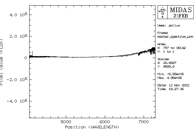
As a test, the combined spectrum can be plotted (a more sophisticated plotting option is described below) with following commands:

 crea/grap
 plot/axes 4000,8000 0,10 0 "wavelength" "relative intensity"
 overplot/row master_spectrum_wrm.fit

Depending on the number of identified orders, the plot range (second row) needs to be adjusted. You also can use this option to zoom in the spectrum. The parameters are

 plot/axes xmin, xmax, ymin, ymax, x axis label, y axis label

4000 - 8000 Angstrom is the usual wavelength range covered by the spectrograph.

The spectrum be be save in the postscript format with

 copy/graph postscript

The file should than be renamed, since the above command always creates files with the name postscript. An example spectrum of the Moon is shown in the following figure.

Spectrum of Mu Pegasi (G8 III)

All the tiny features are real absorption lines and not noise!

Due to the Doppler effect, the relative velocity of a star towards or away from us results in a wavelength shift. This shift can be measured with the help of the absorption lines that are found in the spectrum.

If MIDAS has been closed in the meantime, reopen it first and plot the fully calibrated spectrum:

 crea/graph 
 plot master_spectrum_wrm.fit

The following commands can be used to select a certain range in x (xlow < x < xhigh) or y (ylow < y < yhigh) in the plot to zoom in on one spectral line:

 set/gra xa=xlow,xhigh
 set/gra ya=ylow,yhigh
 plot master_spectrum_wrm.fit

For this purpose, suitable spectral lines must be selected whose rest wavelengths are known.

Please note: If difficulties arise during the line selection, it can be helpful to look at a hydrogen lines for a first estimation. However, since these lines are often very broad, the radial velocity determined in this way will usually not be very accurate. Another pair of lines suitable in many cases would also be seen by pointing the spectrograph at street lamps, although these types of lamps are becoming increasingly rare. Alternatively, you can jump to the Plotting the spectrum section and look at the spectrum divided into smaller sections. This way you may already get a better impression of the potential spectral type and potentially suitable spectral lines.

The central wavelength must now be determined for the selected lines. To achieve this, the line can be fitted with a Gaussian function:

 center/gauss gcursor,2 ? absorption

To do the fit of the function click left and right of the absorption line with the left mouse button, to quit press the right mouse button. In the terminal you will find the fit parameters like “CENTER” (central wavelength of the line core) or “FWHM” (Full Width at Half Maximum), which gives you the width of the Gaussian function. Re-do the measurement several times to be sure to set good limits for the Gaussian fit and to get a feeling of the error in the measurement. This should be done for at least five single absorption lines. Do you see a difference in the accuracy of the measurent of the central wavelength of different lines? Discuss the reason in the report. With the help of the Doppler formula you can then calculate the relative velocity of the star from the shift of the central wavelength of the absorption lines in respective to their rest wavelength. The rest wavelength can be determined via the NIST database. Of course, we also have a tutorial for this.

The radial velocity is usually given with respect to the barycenter, the center of mass of the solar system, to correct out the effect of the Earth's proper motion. The necessary correction can be calculated with the help of the script 2_barycentric_velocity_correction.py. The coordinates of the object, the observation time, the time zone, and the coordinates of the observatory must be specified:

 ##################################################################################
 ############################ Script Parameters ###################################
 ##################################################################################
 
 ################   REPLACE EVERY "?" WITH ITS RESPECTIVE VALUE    ################
 
 ##### Target coordinates #####
 # enter the object's ICRS coordinates
 right_ascension                     = '?h ?m ?s'            # as hour angle: hour | minute | second
 declination                         = '+?deg ?m ?s'         # in deg | arcmin |arcsec
 
 ##### Observation time #####
 observation_date                    = '????-??-?? ??:??:??' # enter the observation date formatted as 'YYYY-MM-DD HH:MM:SS'. 
                                                               Be careful, to enter the correct day if observations were made 
                                                               past midnight!
 time_zone                           = ?                     # type +1 for the central european time zone or +2 when time was 
                                                               switched to daylight saving
 
 ##### Observatory #####
 observatory_latitude                = ?                     # values in degrees, north is positive
 observatory_longitude               = ?                     # values in degrees, east is positive
 observatory_height_above_MSL        = ?                     # enter in meter

As a result you get the barycentric velocity correction in km/s.

Important: Make sure that the virtual environment we used for data reduction is disabled before proceeding:

 deactivate

The spectrum should be plotted by means of the python script 3_printmasterplot.py, which can be found in the following directory ~/scripts/n1_baches/. This script can extract both the total spectrum created by MIDAS and the individual spectra of the various orders from the FITS files and then display them.

The following options must be set in the Python script:

 ############################################################################
 ####          Configuration: modify the file in this section            ####
 ############################################################################
 
 #   Name of file with individual orders
 file_with_orders = "master_spectrum_wr.fit"
 
 #   Name of file with merged spectrum
 file_with_merged_spectrum = "master_spectrum_wrm.fit"
 
 #   Name of the object
 object_name = "?"
 
    
 ###
 #   Radial velocity [km/s]
 #       The specification of the radial velocity is necessary for the
 #       line identification to work correctly (see below).
 radial_velocity = 0.
 
 
 ###
 #   Line identifications
 #
 #   Ions for which line markers are to be drawn.
 #   Example: ["HI", "FeI", ...]
 ions = []
 
 #   Add lines that are not in the default database
 #   Format: {"Element descriptor": [[wavelength, alignment parameter]]}
 #           alignment parameter possibilities: "center", "left", "right"
 manual_lines = {"Example Element": [[0.,"center"]], "Example Element 2": [[0.,"left"]]}
 
 #   Percent the line flux must be lower than the continuum
 percentage_line_flux_must_be_below_continuum = 3.

By default, the script creates two PDF files: spectrum_panels_MIDAS-merged_<objectname>.pdf and spectrum_total_MIDAS-merged_<objectname>.pdf. The file with total in its name displays the spectrum in a single plot. Due to the large spectral range in this plot, details are often hard to see. Therefore, the second file (with panels in the name) shows the respective spectrum distributed over several “panels”, which in turn makes the identification of individual lines much easier.

For possible later reuse, the extracted spectrum is stored as a CSV file in the output folder. The following format is used for the file name: <object_name>_<merge_type>_<panel_number>.csv.

Two example plots for Arcturus and the Sun (Moon) can be found here: Mu Pegasi (G8 III) & Xi Persei (O7.5 III).

The ions that are to be identified via the line identifications must be specified in the variable ions. If this is not done, no line identifications will be displayed! The script reads the line information from the file atomic_lines.tsv. But since this file contains only a selection of spectral lines, which are found in the many different stars, it is necessary to search for additional spectral lines and their transitions, e.g., in the NIST data base as already mentioned, we also have a tutorial for this database. The extracted line information need to be entered into the variable manual_lines.

Using the lines and ions identified in the spectrum, the spectral type can then be easily determined. This graph [1] can be helpful for a first classification of the spectra. Furthermore, the spectra can also be compared with a spectral atlas .

[1] Struve, O. (1959): Elementary Astronomy (Oxford University Press, New York) p. 259

A usual report is to be handed in. See a general overview about the required structure and content here.

For this experiment, the theoretical overview in the report should describe the formation of stellar spectra, the different spectral types with their main characteristics and properties, and the concepts behind radial velocity measurements.

In the methods section describe the observations and the data reduction, highlight points that deviate from general description in here and list all the parameters you set for the extraction. Further, include all the plots of the data reduction in the report (a few in the text, most of them in the appendix).

The results part presents and describes the spectra of the stars (a few selected significant orders of each star are sufficient to be shown here, the rest goes into the appendix). It also includes the measurement of the radial velocity of each star from the line shift (including an error estimate) and the barycentric velocity correction for one of them. Do not forget to list the individual lines that you use with their respective rest frame wavelength, line shift, etc.

The analysis of the spectra contains the estimation of the spectral type for your target stars based on the characteristics that you have described in the theoretical background section.

Finally, discuss your findings. Bring your results into a larger context and make a literature comparison when possible. This also includes that you identify potential problems with the data, the data reduction, or the analysis and possible solutions for them. Are there inconsistencies? Do you see specific and obvious features in the spectra you cannot explain?

Note: The plots of the individual orders are in large files which generally do not fit into an email appendix. You may upload your report to the University cloud system (BoxUP) or send us the path to it on our lab course computer.

Overview: Laboratory Courses