N1 - Stellar spectra of different spectral types (DADOS)

The aim of this observation is to obtain an overview of different spectral types. Thus, we will give you the coordinates and the apparent magnitude of four stars of different spectral type that are well visible during the night of your observation. Take spectra of these stars in order to classify them by means of the spectral lines and the shape of the continua.

Nightly observations at the OST in Golm with the DADOS spectrograph are required. The DADOS with a 900 lines/mm grid is currently used in combination with the QHY 268M. The scientific and technical background for this observation are presented in the seminary talks. A list with objects will be provided by us.

Note: The following exposures are needed for every star:

• stellar spectra
• calibration spectra with a discrete light source
• calibration spectra with a continuous light source (flatfield)
• darkframes

The calibration exposures are needed to calculate the pixel scale (wavelength calibration) and to remove the instrument signatures and possible artifacts.

The scripts needed for the data reduction can be found on the Laboratory computer in the directory ~/scripts/n1_dados/transition_version.

The first tasks are to login to the Laboratory Computer and to copy the observational data (FITS files), including darkframes, and the additional calibration exposures from the directory ~/data/<date> to your own directory ~/data_reduction/.

The 1_masterimages.py script is available for data reduction. This script combines the individual images into corresponding 'master' files. For example, the individual dark images are combined into masterdarks according to exposure time by calculating the median of all images for each pixel.

The following variables need to be set in the script:

###
#   Path to the directories with the images
#
#   Darks:
path_darks: str = '?'
 
#   Flat darks:
path_flat_darks: str = '?'
 
#   Flats:
path_flats: str = '?'
 
#   Darks for wavelength calibration exposures:
path_wavelength_darks: str = '?'
 
#   Wavelength calibration exposures:
path_wavelength: str = '?'
 
#   Spectra:
path_spectra: str = '?'

path_darks is the path to the dark images with the same exposure time as the spectra images. The path to the latter must be specified in path_spectra. The flats must be specified in path_flats and the corresponding darks in path_flat_darks. The same applies to the images for the wavelength calibration, which must be specified under path_wavelength and path_wavelength_darks.

In addition, the variable trim_image should be set to False.

There are several tools for viewing 2D images in FITS format. ds9 is easy to use and can be started from the terminal:

ds9 filename.fit 

Tasks:

• determine the range of camera chip rows that contains the stellar spectrum (master_spectrum.fit).
• determine the range of camera chip rows that can be used as background. Important: The background region must be outside the spectrum, but still within the used slit of the spectrograph. If the latter cannot be distinguished from the black background, compare with the images of the lamp spectra (master_wave.fit).

The script searches for the maxima in the calibration spectrum, marks them and notes the pixel number where the intensity maxima are located. It then assigns a wavelength to each of these values. This creates a pixel-wavelength mapping that is used to analyze the star's spectrum.

The corresponding script is called 2_findcaliblines.py. In this file, using an editor of your choice (e.g. Kate), you only need to edit the line region where the calibration spectrum is to be found (specRegionStart and specRegionEnd; can be the same as the one you want to extract the star spectrum from) and a line region that is outside the slits (bgRegionStart, bgRegionEnd):

# region (rows on the image) containing the calibration spectrum
specRegionStart = 495
specRegionEnd   = 600
 
# background region (rows on the image), which needs to be outside of the slits
bgRegionStart   = 0
bgRegionEnd     = 200

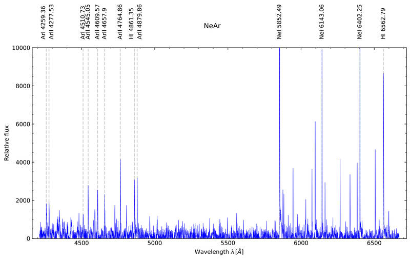
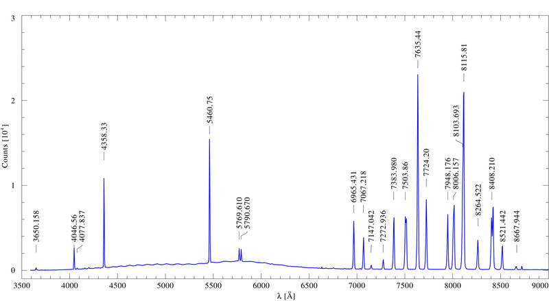
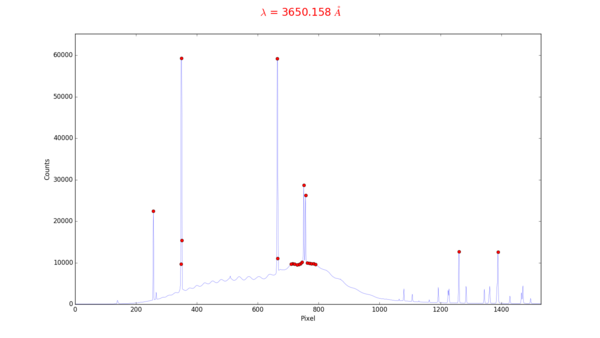
The calibration is designed such that lines of mercury and argon are identified. The strongest lines that can be expected are marked in the following plot.

Emission spectrom of our Ne-Ar calibration lamp. The strongest lines are identified.

Old Hg & Ar calibration

Emission spectrom of our calibration lamp. The strongest mercury and argon lines are identified.

Now run the script by executing:

 python 2_findcaliblines.py

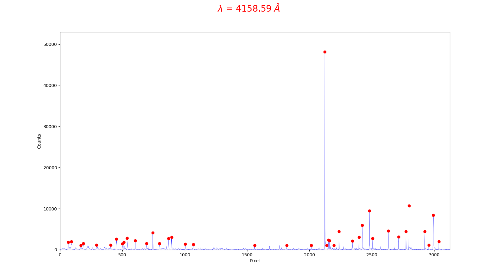
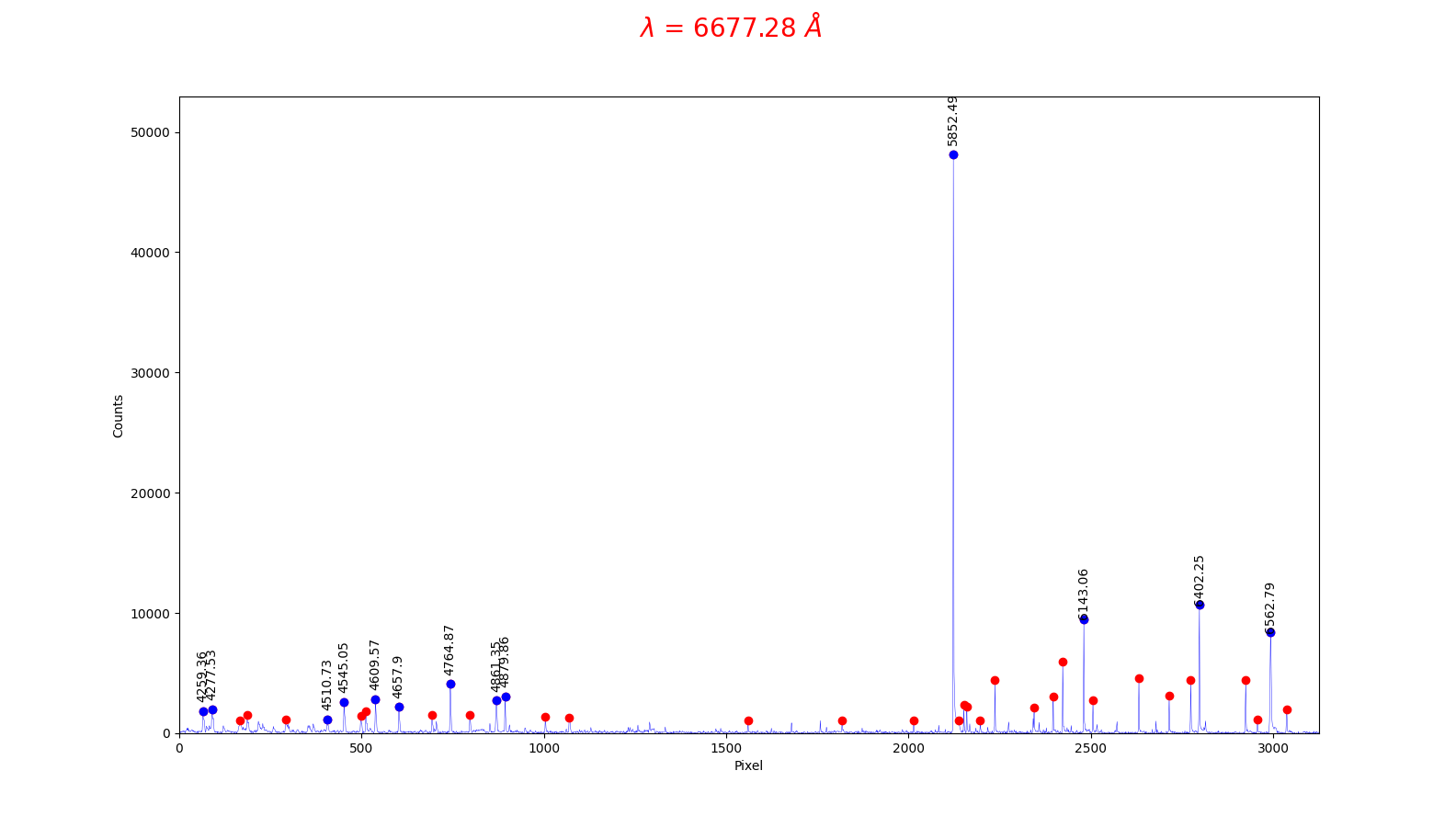
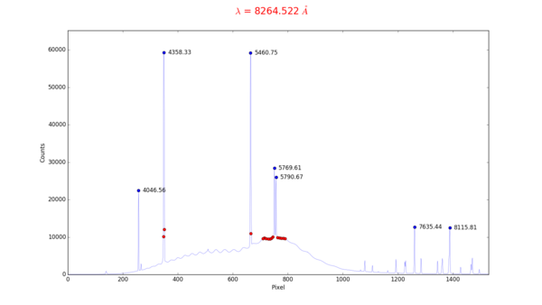
After running the script, the following window will appear, showing the emission line spectrum of neon and argon, with all lines identified by the script marked with a red circle. All emission lines with a known wavelength must now be selected in this window. The example spectrum above with the identified lines is very helpful here. The script specifies the possible lines, so all you need to do is left-click to select the corresponding red circles. The wavelength of the current line is displayed in red at the top of each window. If the wavelength of a line not marked with a red circle is displayed, it can be skipped by right-clicking. Successfully marked lines will then appear in blue and the corresponding wavelength will be written next to the emission peak (see below). At least four lines must be marked for a successful wavelength calibration. Once all possible lines have been marked, the process can be completed by pressing the 'Q' key on the keyboard.

Calibration plot detected lines

Calibration plot with the most prominent lines selected

Old Hg & Ar calibration

Calibration plot detected lines

Calibration plot with seven marked lines

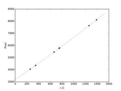
Subsequently, the calibration curve will be plotted by the script (see below). If the calibration procedure is successful, the calibration curve will be nearly linear.

Relation between wavelength and pixel for our DADOS spectrograph

Old Hg & Ar calibration

Relation between wavelength and pixel for our DADOS spectrograph

By default the following files are then created:

• calibration_spectrum.dat - containing the correlated pixel to wavelength scale
• calibration_selection.pdf - a plot showing the selected lines for the wavelength calibration (please add this plot to your report)
• calibration_fit.pdf - a plot of the wavelength calibration (i.e. calibration_spectrum.dat, please add this plot to your report)

Check the plots for possible errors. Especially, if the calibration_fit.pdf does not appear to be linear, edit the script, and run it again. Errors sources could be:

• wrongly marked lines
• a non standard wavelength range or another calibration lamp. The wavelengths of additional calibration lines can be identified with the help of the NIST Database. Those wavelength need be added to the variable linelist in the script.

Once the wavelength-pixel mapping has been determined, the actual star spectrum can be evaluated. By default, the spectrum is divided by the flat field and then the wavelength calibration is performed. It is also possible to normalize the spectrum and mark the spectral lines identified in the spectrum.

This associated script is named 3_extractspectrum.py. The script has a number of parameters, similar to the previous scripts, along with some additional parameters. The parameter section usually looks like this:

#   Name of the object
object_name: str = "star"
 
###
#   Extraction regions
#
#   Region containing the science spectrum
spec_region_start: int = 759
spec_region_end: int = 772
 
#   Sky background region (inside the slit)
background_sky_start: int = 710
background_sky_end: int = 730
 
###
#   Plot range
#
#   Set the variables to '?' for an automatic resizing
lambda_min: str | float = '?'
lambda_max: str | float = '?'
flux_min: str | float = '?'
flux_max: str | float = '?'
 
###
#   Normalization ?
#   Possibilities: True or False
#
normalize: bool = False

Comments on these parameters:: The name of the observed star can be specified in object_name. The variables spec_region_start and spec_region_end define the lines of the camera chip containing the spectrum to be read out. From this star spectrum the sky background has to be subtracted. This is done by selecting a region that lies within the slit but does not contain a spectrum. This region is defined by the variables background_sky_start and background_sky_end. The options lambda_min and lambda_max as well as flux_min and flux_max can be used to restrict the plot area on the X or Y axis. If ? is written in these variables, the plot range is automatically defined.

Now run the script:

 python 3_extractspectrum.py

The following files are generated by default:

• spectrum_panels_{object_name}.pdf - with the spectrum in several panels (zoom version)
• spectrum_total_{object_name}.pdf - with the spectrum displayed in a single panel
• {object_name}_spectrum_total.dat - with the spectrum in tabular form
• {object_name}_spectrum_total.csv - with the tabulated spectrum in CSV format

Line identifications for known spectral lines can be plotted by means of a file containing these information. The ions that are to be identified via the line identifications must be specified in the variable ions. If this is not done, no line identifications will be displayed! The script reads the line information from the file atomic_lines.tsv. But since this file contains only a selection of spectral lines, which are found in the many different stars, it is necessary to search for additional spectral lines and their transitions, e.g., in the NIST data base as already mentioned, we also have a tutorial for this database. The extracted line information need to be entered into the variable manual_lines.

The following options must be set in the Python script:

A usual report is to be handed in. See a general overview about the required structure and content here.

For this experiment, the theoretical overview in the report should describe the formation of stellar spectra, the different spectral types with their main characteristics and properties, and the concepts behind radial velocity measurements.

In the methods section describe the observations and the data reduction, highlight points that deviate from general description in here and list all the parameters you set for the extraction. Further, include all the plots of the data reduction in the report (a few in the text, most of them in the appendix).

The results part presents and describes the calibrated spectra of the stars.

The analysis of the spectra contains the estimation of the spectral type for your target stars based on the characteristics that you have described in the theoretical background section.

Finally, the results are discussed and placed in a wider context. This includes, for example, a comparison with the literature where possible. Possible sources of error should also be discussed. Are there inconsistencies in the data or deviations from what is expected? Or are there structures and anomalies in the spectra that cannot be explained? Describe possible solutions and explanations for the problems found.

Note: This figure [1] can be helpful to classify the spectra. You may also compare your spectra to the spectral atlas and look up the NIST web page to identify individual spectral features. Another guide to the classification of stellar spectra can be found here.

Note: The plots of each order of the spectra can be large files, often too large for an email attachment. You can upload the report to the University Cloud Service (BoxUP) and send us the link or file path to the plots if you have saved them on the lab computer.

[1] Struve, O. (1959): Elementary Astronomy (Oxford University Press, New York) p. 259

Overview: Laboratory Courses