N1 - Stellar spectra of different spectral types (DADOS)
The aim of this observation is to obtain an overview of different spectral types. Thus, we will give you the coordinates and the apparent magnitude of four stars of different spectral type that are well visible during the night of your observation. Take spectra of these stars in order to classify them by means of the spectral lines and the shape of the continua.
Observation
Nightly observations at the OST in Golm with the DADOS spectrograph are required. The scientific and technical background for this observation are presented in the seminary talks. A list with objects will be provided by us.
Note: The following exposures are needed for every star:
- the stellar spectra
- calibration spectra with a discrete light source
- calibration spectra with a continuous light source (flatfield)
- darkframes for the exposures of the stellar spectra and the continuous light source
The calibration exposures are needed to calculate the pixel scale (wavelength calibration) and to remove the instrument signatures and possible artifacts.
Data reduction
The scripts needed for the data reduction can be found on the Laboratory computer in the directory ~/scripts/n1_dados.
Selection and inspection of the data
The first tasks are to login to the Laboratory Computer and to copy the observational data (FITS files), including darkframes, and the additional calibration exposures from the directory ~/data/<date> to your own directory ~/data_reduction/. There are different tools to view the FITS files (two dimensional CCD images or data tables). ds9 is easy to handle and can be started from the terminal via:
ds9 filename.fit
Tasks:
- determine the range of CCD rows that contains the stellar spectrum
- determine the range of CCD rows that can be used as background. Important: The background region must be outside the spectrum, but still within the used slit of the spectrograph. If the latter cannot be distinguished from the black background, compare with the images of the lamp spectra.
Wavelength calibration
Basic principle
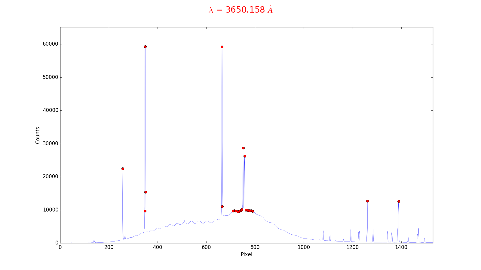
This script finds the maxima of the emission lines in the discrete calibration spectrum, marks them, and identifies their pixel number (i.e. position of the maximum). These numbers are correlated to the wavelengths of those emission lines to have the conversion scale between the pixel and the wavelength.
Parameter
The required script (1_findcaliblines.py) is written in Python. Edit the file using a text editor of your choice (i.e. kate or emacs) and adjust the path to the exposure of the discrete light source (the black lamp that emits the line spectrum) as well as the CCD rows that should be extracted. Two row ranges are requested. One that contains the calibration spectrum and hence should lie within the slit, while the second one is designated for a background region and therefore needs to lie outside the slit:
# name of the file with the wavelength calibration spectrum
calibFileName   = "calib_wave.FIT"

# region (rows on the image) containing the calibration spectrum
specRegionStart = 495
specRegionEnd   = 600

# background region (rows on the image), which needs to be outside of the slits
bgRegionStart   = 0
bgRegionEnd     = 200
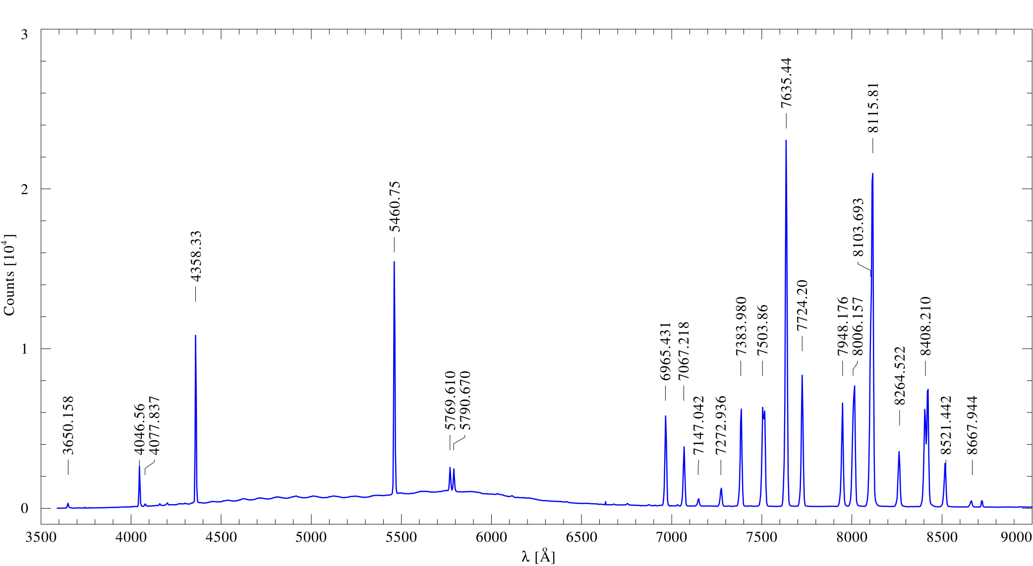
The calibration is designed such that lines of mercury and argon are identified. The strongest lines that can be expected are marked in the following plot.
Execution of the script
Now run the script by executing:
python 1_findcaliblines.py
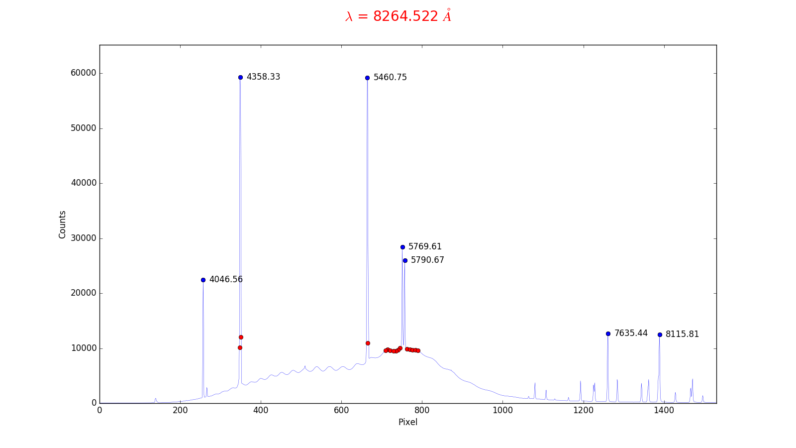
Afterwards the following window will be displayed on the screen, showing the mercury and argon emission line spectrum. All lines that were identified by the script are highlighted by a red circle. Now, all lines with known wavelengths need to be marked. For this task, the above example spectrum can be very useful. The script runs through a list of predefined lines. The wavelength of the current line is displayed in the upper part of the window. The line corresponding to this wavelength can now easily marked by clicking into the corresponding red circle with the left mouse button. This circle should now appear blue and the corresponding wavelength is written next to the line peak (see below). If a wavelength is displayed that does not correspond to any of the highlighted lines, this wavelength can be skipped with a right click. At least four lines need to be marked to facilitate a successful wavelength calibration. If all useful lines are marked, this procedure can be completed by pressing the Q key on the keyboard.
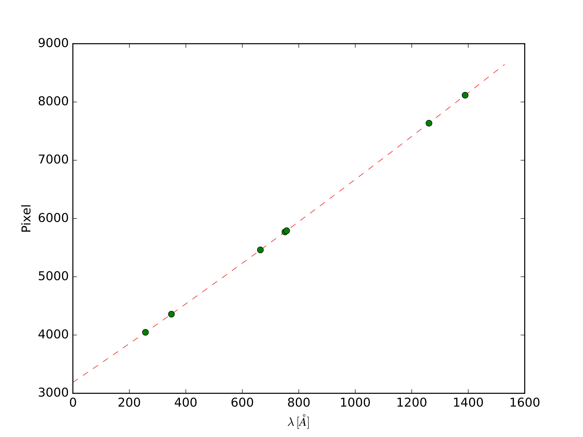
Subsequently, the calibration curve will be plotted by the script (see below). If the calibration procedure is successful, the calibration curve will be nearly linear.
By default the following files are then created:
calibration_spectrum.dat- containing the correlated pixel to wavelength scalecalibration_selection.pdf- a plot showing the selected lines for the wavelength calibration (please add this plot to your report)calibration_fit.pdf- a plot of the wavelength calibration (i.e.calibration_spectrum.dat, please add this plot to your report)
Error handling
Check the plots for possible errors. Especially, if the calibration_fit.pdf does not appear to be linear, edit the script, and run it again. Errors sources could be:
- wrongly marked lines
- a non standard wavelength range or another calibration lamp. The wavelengths of additional calibration lines can be identified with the help of the NIST Database. Those wavelength need be added to the variable
linelistin the script.
The stellar spectrum
Basic principle
The next step after the determination of the calibration curve is the reduction of the stellar spectrum. First, the darkframe is subtracted from the spectrum, then the spectrum is divided by the flatfield, and, lastly, the wavelength calibration is performed. It also exist the possibility to mark spectral lines in the spectrum.
Parameters
This associated script is named 2_extractspectrum.py. The script has a number of parameters, similar to the previous scripts, along with some additional parameters. The parameter section usually looks similar to this:
 ### science spectrum file ###
 # file with stellar spectrum
 science        =  'star.FIT'
 # directory of the darkframe for the stellar spectrum
 darkframe_dir  =  'darks/??s/'
 # flatfield directory
 flatfield_dir  =  'flats/'
 # directory of the darkframe for the flats
 flatdark_dir   =  'darks/??s/'


 ### Data that should be extracted  ###
 # region containing the science spectrum
 specRegionStart = 495
 specRegionEnd   = 590

 # sky background region (inside the slit)
 bgSkyStart   = 96
 bgSkyEnd     = 104


 ### Plot range ###
 # set the variables to '?' for an automatic resizing
 lambdamin = '?'
 lambdamax = '?'
 #lambdamin = 3500.
 #lambdamax = 5000.
Comments on these parameters::
- The variables
specRegionStartandspecRegionEnddefine the range of CCD rows that will be extracted. These rows need to be chosen such that the stellar spectrum is completely covered. - The sky background needs to be subtracted. So, as before, a range of rows within the slit but outside the spectrum must be chosen. If possible, the number of rows should be the same for both, i.e. (specRegionStart - specRegionEnd) = (bgSkyStart - bgSkyEnd).
- The options
lambdaminandlambdamaxcan be used to restrict the plot range. If these variables contain a?the plot range will be determined automatically.
Execution of the script
Now run the script:
python 2_extractspectrum.py
The following files are then created:
- stern_spectrum.dat - with the tabulated spectrum
- stern_spectrum.pdf - showing the plotted spectrum
- flatfield.pdf - showing the plotted flatfield (please add this plot to your report)
Identification of spectral lines
Line identifications for known spectral lines can be plotted by means of a file containing these information. An example file (absorption_lines) can be found in the scripts directory. This file contains some but not all important spectral lines that are visible in the variety of stars, which we observe. Therefore, it is required to search for additional spectral lines and the corresponding transitions for example in the NIST Database. A how-to for this can be found here. Moreover, it is recommended to create an individual line-identification file for each of the observed stars.
To identify lines in the stellar spectrum, copy the relevant lines into the separate file. The format of that file should look like (wavelength in Å | identifier):
 3888.052	HI
 3970.075	HI
 4861.38	HI
 6562.88	HI
 5801.33	5811.98	CIV
As can be seen from the last entry, also ions with multiplet transitions can be included. Line identifications that can be not assigned to any spectral line need to be removed from the corresponding file.
The file can then be referenced in the Python script:
 # file containing line identifications
 lineFile = "directory/line_list_for_starname.dat"
Rerun the script to obtain a plot with adjusted line identifications.
Report
A usual report is to be handed in. See a general overview about the required structure and content here.
For this experiment, the theoretical overview in the report should describe the formation of stellar spectra, the different spectral types with their main characteristics and properties, and the concepts behind radial velocity measurements.
In the methods section describe the observations and the data reduction, highlight points that deviate from general description in here and list all the parameters you set for the extraction. Further, include all the plots of the data reduction in the report (a few in the text, most of them in the appendix).
The results part presents and describes the calibrated spectra of the stars.
The analysis of the spectra contains the estimation of the spectral type for your target stars based on the characteristics that you have described in the theoretical background section.
Finally, discuss your findings. Bring your results into a larger context and make a literature comparison when possible. This also includes that you identify potential problems with the data, the data reduction, or the analysis and possible solutions for them. Are their inconsistencies? Do you see specific and obvious features in the spectra you cannot explain?
Note: This figure [1] can be helpful to classify the spectra. You may also compare your spectra to the spectral atlas and look up the NIST web page to identify individual spectral features. Another guide to the classification of stellar spectra can be found here.
[1] Struve, O. (1959): Elementary Astronomy (Oxford University Press, New York) p. 259